From 20997ae6926d589b7b964d7dcc60f1722ae1d136 Mon Sep 17 00:00:00 2001
From: Adrian Kummerlaender
Date: Thu, 23 Sep 2021 23:19:45 +0200
Subject: Add article on noise in ray marching
---
articles/2021-09-26_noise_and_ray_marching.org | 276 +++++++++++++++++++++
flake.lock | 8 +-
.../2021-09-26_noise_and_ray_marching.org | 1 +
tags/english/2021-09-26_noise_and_ray_marching.org | 1 +
tags/math/2021-09-26_noise_and_ray_marching.org | 1 +
5 files changed, 283 insertions(+), 4 deletions(-)
create mode 100644 articles/2021-09-26_noise_and_ray_marching.org
create mode 120000 tags/development/2021-09-26_noise_and_ray_marching.org
create mode 120000 tags/english/2021-09-26_noise_and_ray_marching.org
create mode 120000 tags/math/2021-09-26_noise_and_ray_marching.org
diff --git a/articles/2021-09-26_noise_and_ray_marching.org b/articles/2021-09-26_noise_and_ray_marching.org
new file mode 100644
index 0000000..d3b231d
--- /dev/null
+++ b/articles/2021-09-26_noise_and_ray_marching.org
@@ -0,0 +1,276 @@
+* Noise and Ray Marching
+[[https://literatelb.org][LiterateLB's]] volumetric visualization functionality relies on a simple ray marching implementation
+to sample both the 3D textures produced by the simulation side of things and the signed distance
+functions that describe the obstacle geometry. While this produces surprisingly [[https://www.youtube.com/watch?v=n86GfhhL7sA][nice looking]]
+results in many cases, some artifacts of the visualization algorithm are visible depending on the
+viewport and sample values. Extending the ray marching code to utilize a noise function is
+one possibility of mitigating such issues that I want to explore in this article.
+
+While my [[https://www.youtube.com/watch?v=J2al5tV14M8][original foray]] into just in time visualization of Lattice Boltzmann based simulations
+was only an aftertought to [[https://tree.kummerlaender.eu/projects/symlbm_playground/][playing around]] with [[https://sympy.org][SymPy]] based code generation approaches I have
+since put some work into a more fully fledged code. The resulting [[https://literatelb.org][LiterateLB]] code combines
+symbolic generation of optimized CUDA kernels and functionality for just in time fluid flow
+visualization into a single /literate/ [[http://code.kummerlaender.eu/LiterateLB/tree/lbm.org][document]].
+
+For all fortunate users of the [[https://nixos.org][Nix]] package manager, tangling and building this from the [[https://orgmode.org][Org]]
+document is as easy as executing the following commands on a CUDA-enabled NixOS host.
+
+#+BEGIN_SRC sh
+git clone https://code.kummerlaender.eu/LiterateLB
+nix-build
+./result/bin/nozzle
+#+END_SRC
+
+** Image Synthesis
+The basic ingredient for producing volumetric images from CFD simulation data is to compute
+some scalar field of samples \(s : \mathbb{R}^3 \to \mathbb{R}_0^+\). Each sample \(s(x)\) can be assigned a color
+\(c(x)\) by some convenient color palette mapping scalar values to a tuple of red, green and blue
+components.
+
+[[https://literatelb.org/tangle/asset/palette/4wave_ROTB.png]]
+
+The task of producing an image then consists to sampling the color field along a ray assigned
+to a pixel by e.g. a simple pinhole camera projection. For this purpose a simple discrete
+approximation of the volume rendering equation with constant step size \(\Delta x \in \mathbb{R}^+\) already
+produces suprisingly good pictures. Specifically
+$$C(r) = \sum_{i=0}^N c(i \Delta x) \mu (i \Delta x) \prod_{j=0}^{i-1} \left(1 - \mu(j\Delta x)\right)$$
+is the color along ray \(r\) of length \(N\Delta x\) with local absorption values \(\mu(x)\). This
+local absorption value may be chosen seperately of the sampling function adding an
+additional tweaking point.
+
+#+BEGIN_EXPORT html
+
+#+END_EXPORT
+
+The basic approach may also be extended arbitrarily, e.g. it is only the inclusion of a couple
+of phase functions away from being able [[https://tree.kummerlaender.eu/projects/firmament/][recover the color produced by light travelling through the participating media that is our atmosphere]].
+
+** The Problem
+There are many different possibilities for the choice of sampling function \(s(x)\) given the results of a
+fluid flow simulation. E.g. velocity and curl norms, the scalar product of ray direction and shear layer
+normals or vortex identifiers such as the Q criterion
+\[ Q = \|\Omega\|^2 - \|S\|^2 > 0 \text{ commonly thresholded to recover isosurfaces} \]
+that contrasts the local vorticity and strain rate norms. The strain rate tensor \(S\) is easily
+recovered from the non-equilibrium populations \(f^\text{neq}\) of the simulation lattice — and is in
+fact already used for the turbulence model. Similarly, the vorticity \(\Omega = \nabla \times u\) can be
+computed from the velocity field using a finite difference stencil.
+
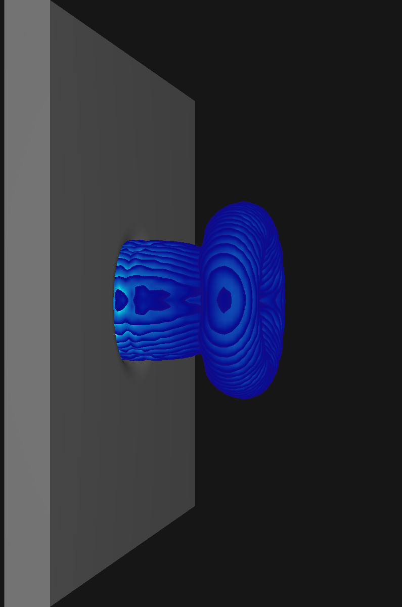
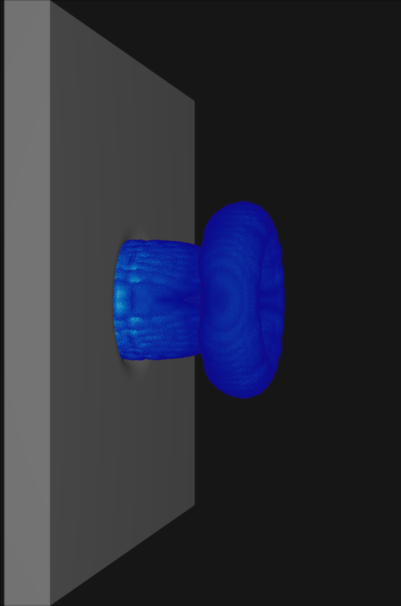
+The problem w.r.t. rendering when thresholding sampling values to highlight structures in the flow
+becomes apparent in the following picture:
+
+#+BEGIN_EXPORT html
+
+
+
Q Criterion
+
+
+
+
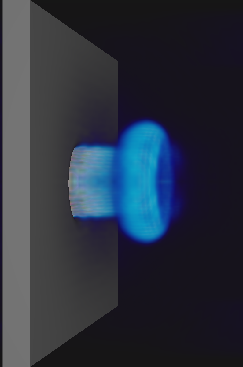
Curl Norm
+
+
+
+
+
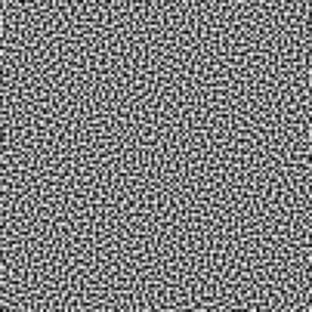
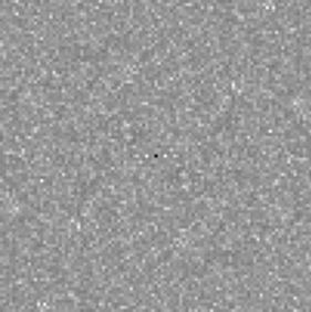
Blue noise texture
+
+
+
+
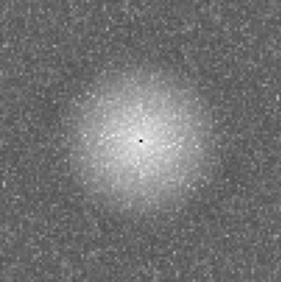
Fourier transformation
+
+
+
+
+
White noise texture
+

+
+
+
Fourier transformation
+
+
+
+
+
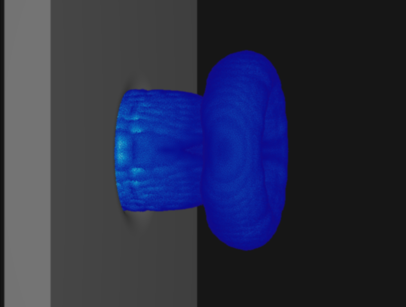
Simple ray marching
+
+
+
+
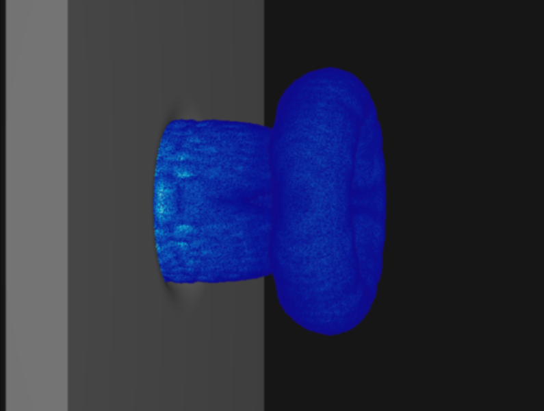
Ray marching with blue noise jittering
+
+
+
+
+
Blue noise
+
+
+
+
White noise
+
+
+